Search capability is ingrained into our daily life. Arguments are commonly ended with the conclusion, “just google it”. Users have come to expect that nearly every application and website provide some type of search functionality. With effective search becoming ever-increasingly relevant (pun intended), finding new methods and architectures to improve search results is critical for architects and developers. Starting from the basics, this blog post will describe AI-powered search capabilities within Redis that utilize vector embeddings created by deep learning models.
This blog post was originally published on MLOps.community and was written on behalf of Redis.
Disclaimer: I work for Redis.
Vector Embeddings
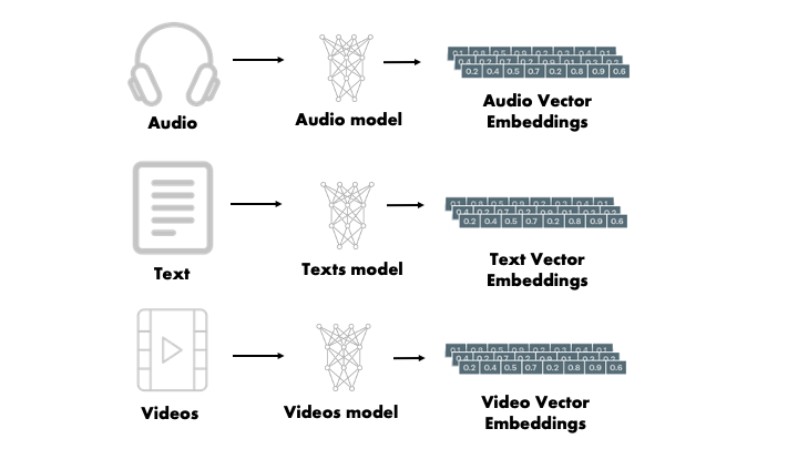
What is a vector embedding? Simply put, vector embeddings are lists of numbers that can represent many types of data.
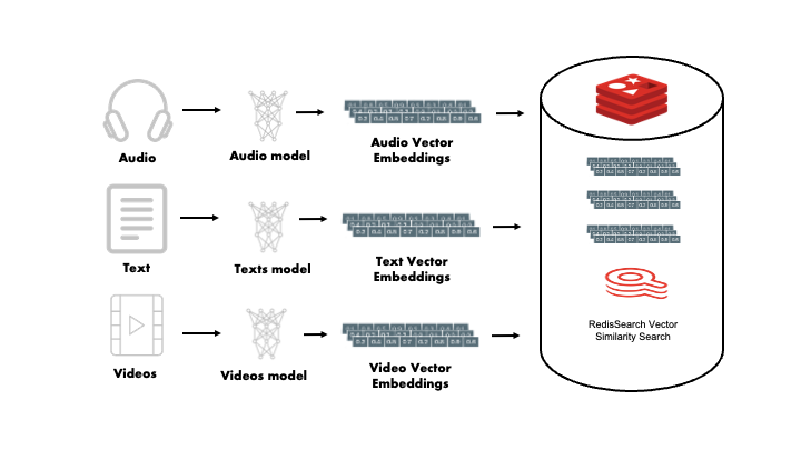
Vector embeddings are quite flexible. Audio, video, text, and images can all be represented as vector embeddings. This quality makes vector embeddings the swiss-army knife of the data scientist’s toolkit.
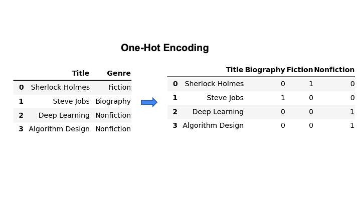
To explain why embeddings provide such utility, let us look at prior methods for dealing with text data such as categorical values in tabular data. Data scientists sometimes utilize methods like one-hot encoding to transform categorical features into numerical values. These encodings would create a column for every type of category. A value of 1 means the item belongs to the category specified by that column. Inversely, a value of 0 signifies the item does not belong to that category.
For example, consider book genres: “Fiction”, “Nonfiction”, and “Biography”. Each of these genres could be encoded into one-hot vectors, however, such vectors would be very sparse as books often don’t belong to more than a couple genres. The figure below shows how this encoding would work. Notice there are twice as many zeros as there are ones. For a category like book genres, this sparsity will become exponentially worse as more genres are added to the dataset.
Sparsity can present challenges for ML models. With each new genre, the representation of the encoding grows in size, and hence the dataset can become computationally expensive to utilize.
For Book genres, or any categorical data with a relatively small number of categories, we may be able to get away with simple one-hot encoding, however, what about the entire English language? Such encoding methods would become impractical with a corpus of that size.
Enter vector embeddings.
Vector embeddings present a fixed size representation that does not grow with the number of observations in the data. The resultant vector created by a model, usually something like 384 floating point values, is significantly more dense of a representation than other encoding methods like one-hot encoding. This means more information is present in less bytes and hence is computationally less expensive to utilize. As you’ll read later, these dense representations can be used for a multitude of purposes such as reverse image search, chatbots, Q&A, and recommendation systems.
Creating Vector Embeddings
In order to understand how vector embeddings are created, a brief introduction to modern Deep Learning models is helpful.
Machine Learning models do not consume unstructured data. In order for a model to understand text or images, we must transform them into a numerical representation. Prior to Machine Learning, such representations were often created “by hand” through Feature Engineering.
With the advent of Deep Learning, non-linear feature interactions in complex data are learned by the model instead of being engineered manually. When an input traverses through a Deep Learning model, new representations of that input data are created in different shapes and sizes. Each layer often focuses on a different aspect of the input. This aspect of Deep Learning, “automatically” generating feature representations from inputs, forms the foundation of how vector embeddings are created.
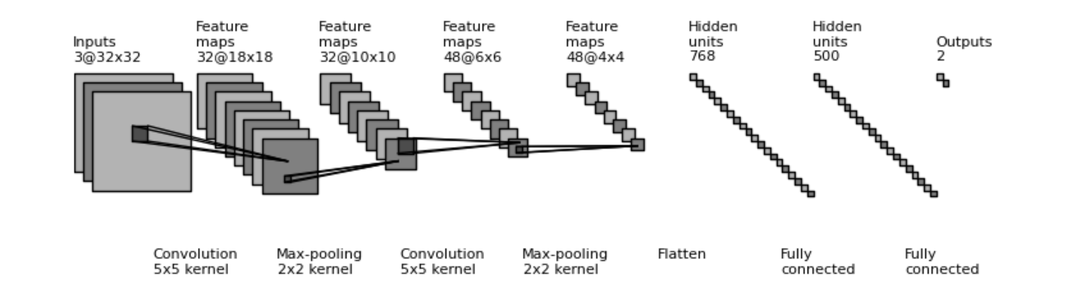
For example, consider the famous ResNet model trained on the ImageNet dataset. ResNet is a Convolutional Neural Network (CNN) commonly used for image-related tasks. In this case, ResNet is trained to predict which of 1000 classes that an object in an image belongs to.
During training, ResNet will capture feature information present in the image by passing it through a number of convolutional, pooling and fully connected layers. The layers will capture features like edges, lines, and corners and group them into “buckets” that are passed to the following layer. Because of the space invariant quality of CNN’s, it doesn’t matter where an edge or line appears in the image, these features will always be mapped to the same bucket. These layers will become successively smaller through the layers of the model until a fully connected layer of 1000 floating point values is presented as the output. Each value represents 1 of 1000 classes. The higher the value, the greater the probability the object in an image belongs to that class.
ResNet, and other image classification models like it, answers the question: “what type of object is in this image?”. However, these classifications are less useful to answer prompts such as: “What images are similar to this image?”. For this question, we need to compare the images together. Despite not being trained for specifically this task, ResNet is still useful as it can capture a dense representation of an image.
Simply put, CNN’s and other models like it, learn useful representations of data in order to perform tasks like image classification. These representations can be extracted while an input is passing through the layers of a model. The extracted layer, also referred to as a latent space, is usually a layer close to the output of the model. In the figure above, this could be the layers with 768, or 500 hidden units. The extracted layer, or latent space, provides a dense representation packed with information about present features that is computationally feasible for tasks like visual similarity search.
This is our vector embedding.
A wealth of pre-trained models exist that can easily be used for creating vector embeddings. The Huggingface Model Hub contains many models that can created embeddings for different types of data. For example, the all-MiniLM-L6-v2 Model is hosted and runnable online, no expertise or install required.
Packages like sentence_transformers, also from HuggingFace, provide easy-to-use models for tasks like semantic similarity search, visual search, and many others. To create embeddings with these models, only a few lines of Python are needed: 1
from sentence_transformers import SentenceTransformer
model = SentenceTransformer('sentence-transformers/all-MiniLM-L6-v2')

sentences = [
  "That is a very happy Person",
  "That is a Happy Dog",
  "Today is a sunny day"
]
embeddings = model.encode(sentences)
Vector Embeddings for Semantic Similarity Search
Semantic Similarity Search is the process by which pieces of text are compared in order to find which contain the most similar meaning. While this might seem easy for an average human being, languages are quite complex. Distilling unstructured text data down into a format that a Machine Learning model can understand has been the subject of study for many Natural Language Processing researchers.
Vector Embeddings provide a method for anyone, not just NLP researcher or data scientists, to perform semantic similarity search. They provide a meaningful, computationally efficient, numerical representation that can be created by pre-trained models “out of the box”. Below, an example of semantic similarity is shown that outlines the vector embeddings created with the sentence_transformers library shown above.
Let’s take the following sentences:
- “That is a happy dog”
- “That is a very happy person”
- “Today is a sunny day”
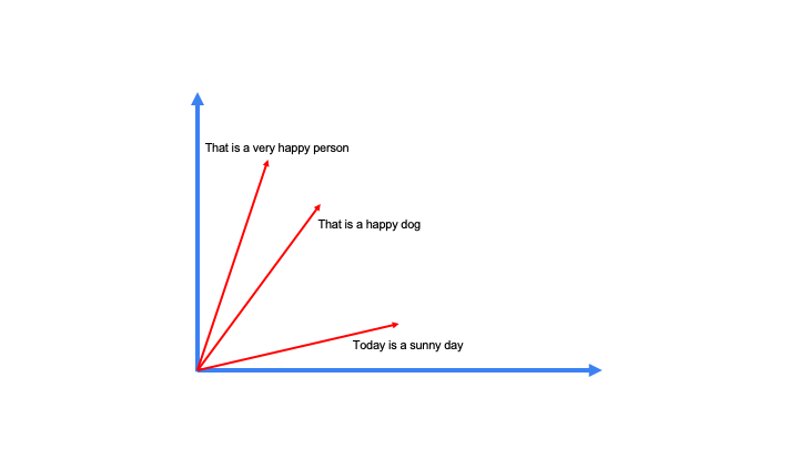
Each of these sentences can be transformed into a vector embedding. Below, a simplified representation highlights the position of these example sentences in 2-dimensional vector space relative to one another. This is useful in order to visually gauge how effective our embeddings represent the semantic meaning of text. More on that below.
Assume we want to compare these sentences to “That is a happy person”. First, we create the vector embedding for the query sentence.
from sentence_transformers import SentenceTransformer
model = SentenceTransformer('sentence-transformers/all-MiniLM-L6-v2')

# create the vector embedding for the query
query_embedding = model.encode("That is a happy person")
Next, we need to compare the distance between our query vector embedding and the vector embeddings in our dataset.
There are many ways to calculate the distance between vectors. Each has their own benefits and drawbacks when it comes to semantic search, but we will save that for a separate post. Below some of the common distance metrics are shown.
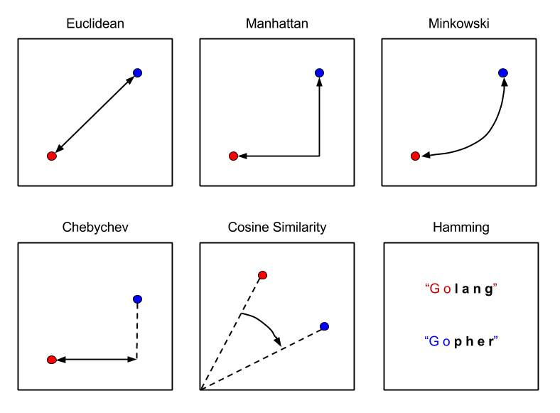
For this example, we will use the cosine similarity which measures the distance between the inner product space of two vectors.
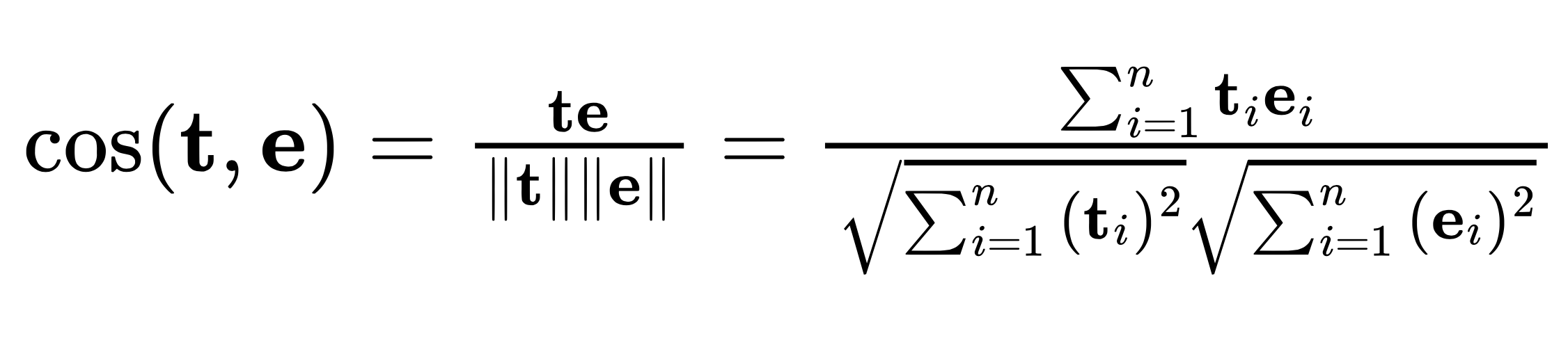
In Python, this looks like
def cosine_similarity(a, b):
    return np.dot(a, b)/(norm(a)*norm(b))
Running this calculation between our query vector and the other three vectors in the plot above, we can determine how similar the sentences are to one another.
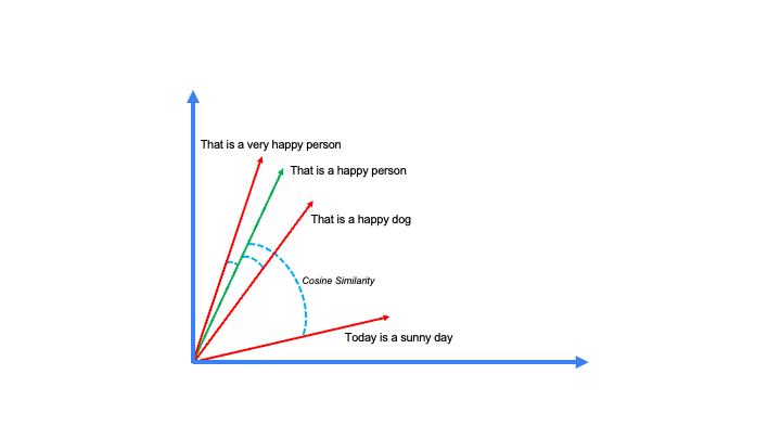
As you might have assumed, “That is a very happy person” is the most similar sentence to “That is a happy person”. This example captures only one of many possible use cases for vector embeddings: Semantic Similarity Search
The Python code to run this entire example is listed below
import numpy as np

from numpy.linalg import norm
from sentence_transformers import SentenceTransformer

# Define the model we want to use (it'll download itself)
model = SentenceTransformer('sentence-transformers/all-MiniLM-L6-v2')

sentences = [
  "That is a very happy person",
  "That is a happy dog",
  "Today is a sunny day"
]

# vector embeddings created from dataset
embeddings = model.encode(sentences)

# query vector embedding
query_embedding = model.encode("That is a happy person")

# define our distance metric
def cosine_similarity(a, b):
    return np.dot(a, b)/(norm(a)*norm(b))

# run semantic similarity search
print("Query: That is a happy person")
for e, s in zip(embeddings, sentences):
    print(s, " -> similarity score = ",
         cosine_similarity(e, query_embedding))
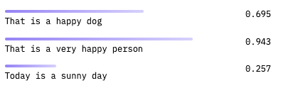
After installing NumPy and sentence_transformers, running this script should result in the following calculations
>>> Query: That is a happy person

>>> That is a very happy person -> similarity score = 0.94291496
>>> That is a happy dog -> similarity score = 0.69457746
>>> Today is a sunny day -> similarity score = 0.25687605
The results of this script should line up with the results that you see on the HuggingFace inference API for the model chosen.
Vector Embeddings for Search In Production
Now, I’d love to say “that’s it” and go build this capability into your platform, however, as many engineers realize every day, development and production are two different beasts. After learning a bit more you may start asking questions like:
- Where do I store these vectors?
- What should the API look like?
- How do I combine this with my traditional search capability like filtering?
Luckily, the good folks at Redis decided to figure out these questions for you and build Vector Similarity Search (VSS) functionality into the existing RediSearch module. This essentially turns Redis into a low-latency, vector database.
The VSS capability is built as a new feature of the RediSearch module. It allows developers to store a vector just as easily as any other field in a Redis hash. It provides advanced indexing and search capabilities required to perform low-latency search in large vector spaces, typically ranging from tens of thousands to hundreds of millions of vectors distributed across a number of machines.
Redis now supports two types of vector indexing:
- Flat
- Hierarchical Navigable Small Worlds (HNSW)
As well as 3 distances metrics:
LP– Euclidean DistanceIP– Inner ProductCOSINE– Cosine Similarity (Like the example shown above)
Below is an example of creating an index with redis-py after the vectors have been loaded into Redis.
from redis import Redis
from redis.commands.search.field import VectorField, TagField

def create_flat_index(redis_conn: Redis, number_of_vectors: int, distance_metric: str='COSINE'):

	image_field = VectorField("img_vector","FLAT", {
        "TYPE": "FLOAT32",
        "DIM": 512,
        "DISTANCE_METRIC": distance_metric,
        "INITIAL_CAP": number_of_vectors,
        "BLOCK_SIZE": number_of_vectors})
	redis_conn.ft().create_index([image_field])
Indexes only need to be created once and will automatically re-index as new hashes are stored in Redis. After vectors are loaded into Redis and the index has been created, queries can be formed and executed for all kinds of similarity-based search tasks.
Indexes only need to be created once and will automatically re-index as new hashes are stored in Redis. After vectors are loaded into Redis and the index has been created, queries can be formed and executed for all kinds of similarity based search tasks.
Better still, all of the existing RediSearch features like text, tag and geographic based search can work together with the VSS capability. This is called hybrid queries. With hybrid queries, traditional search functionality can be used as a pre-filter for vector search which can help bound the search space.
The above index creation function (create_flat_index) can easily be adapted to support hybrid queries by adding new fields such as the TagField or TextField from redis-py.
Try it Out! -> Redis VSS Demo
Recently, I built a web application to explore these capabilities. The Fashion Product Finder utilizes the new VSS capability in Redis along with my other favorite pieces of the Redis ecosystem like redis-om-python. You can access the application here.
Once you’ve signed up to use the application, you will be greeted with a page that looks something like the following.

To query similar products by their textual representation, find a product that you like and click the By Text button. Likewise, for querying by visual vector search, click the By Image button on a product.
The hybrid search attributes can be set for both gender and category of product such that when a vector search is performed, the returned items are filtered by those tags. Below is an example of the visual vector search when the black watch in the bottom right corner is selected.

This demo is a fun way to explore the capabilities within Redis VSS, however, that is not the only component of the Redis ecosystem used in the application. In fact, Redis is the only database used by this application, storing both product metadata with RedisJSON, and vector data with RediSearch.
You can check out the entire codebase here. Please star and share if you find it useful!
For more information on VSS within Redis and the RediSearch module you can check out the following resources:
Documentation
Demos
- Visual and Semantic Search with the Amazon Product Dataset
- Vector-based Sentiment Analysis on Financial news
-
All of the code snippets for this blog post can be found on my GitHub profile gists. ↩
Comments